← Interactive lecture worksheet

Keep the clue.
Five visual explanations.

Original SVG teaching assets. These are final frames; the worksheet animates the steps with prediction pauses. Numbers are supplied examples, not trained predictions.

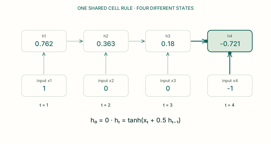
One clue. Many transformations.: final numerical diagram — Scalar RNN: h₀ = 0, input weight 1, bias 0. The four supplied inputs are [1, 0, 0, −1]. This is an arithmetic demonstration, not a trained language model.

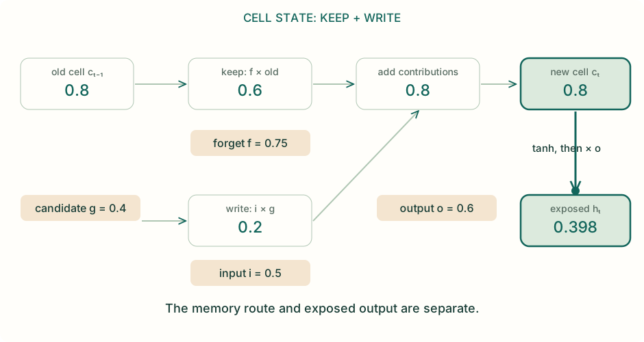
Keep. Write. Reveal.: final numerical diagram — One coordinate of a modern LSTM with forget gate, without peepholes or projection. Gate outputs are manually supplied to isolate the mechanism. Real gates are vectors computed from xₜ and hₜ₋₁. Boundary values 0 and 1 are idealized limits.

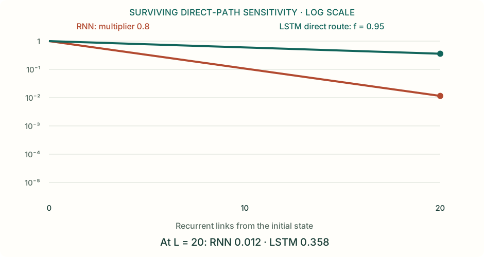
Build a route for credit.: final numerical diagram — Controlled experiment: all write terms are zero, c₀ = h₀ = 1. The RNN comparison is linear with multiplier 0.8. LSTM gates are held constant, so the direct cell-state path has derivative fᴸ. This is not the full recurrent Jacobian or an accuracy measurement.

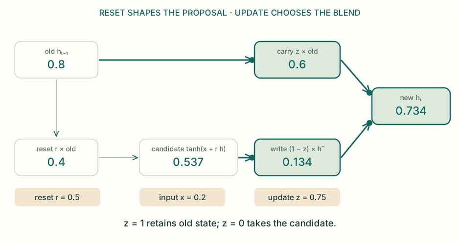
One state. Two gates.: final numerical diagram — Scalar reset-before-matrix GRU: x = 0.2, hₜ₋₁ = 0.8, input/recurrent weights 1 and bias 0. Here z is the fraction of OLD state retained. Some references swap z and 1 − z; some frameworks place reset after the recurrent projection.

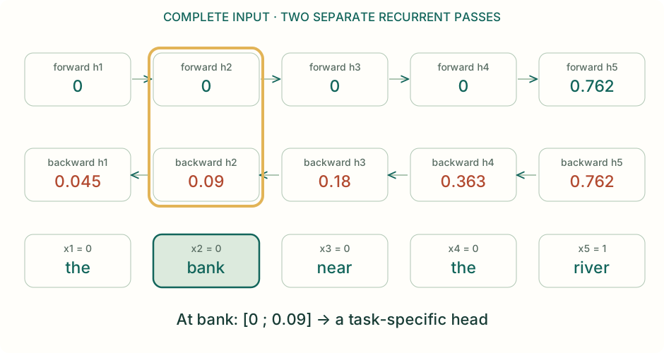
Read both ways. Meet at the same word.: final numerical diagram — The sentences motivate ambiguity; the numbers are a supplied toy encoding, not learned semantics. x = [0, 0, 0, 0, ±1], scalar tanh cells, recurrent weight 0.5, zero boundary states. The two directions use separate parameter sets (chosen equal here for simplicity).