DEEP LEARNINGPresentation & practice sheets
0 of 15 checks understood
← All worksheets
LECTURE PRESENTATION / LSTM · GRU · BIDIRECTIONAL RNNs

Keep the clue.
Read the context.

A useful clue arrives early. The answer comes much later. How can a network decide what to keep—and which direction to read?

90–110 minutes5 guided visual lessons15 checks + design challengeNo coding required
01 / ANTICIPATE

Commit to a prediction before the reveal.

02 / TRACE

Follow the arrows and the numbers.

03 / EXPLAIN

Change one control. Explain what changed.

TODAY’S MISSION · A SMALL EXPERIMENT

Hold one word in mind.
We will need it after the distractions.

Remember this cueBLUE

Hide it. Count backward from 30 in threes. What would make you keep this word while ignoring the numbers?

A plain RNN repeatedly rewrites a fixed-size summary. Today we ask:

  1. Can it protect useful memory while new inputs arrive?
  2. Can a simpler cell make similar decisions?
  3. Can later context help interpret an earlier word—and when is it allowed?

The human-memory exercise is a hook, not a claim that brains implement LSTMs. Gate diagrams are numerical teaching models, not accuracy benchmarks.

Trace an LSTMSeparate keeping, writing and exposing; distinguish c from h.
Compare a GRUExplain reset and update, and compute one state transition.
Choose the contextAlign both directions and detect future-information leakage.

New to sequences? Start with lesson 01. Bring only vectors, multiplication, addition and the idea of gradient descent. The foldouts introduce derivatives and matrix shapes when needed.

01
THE BRIDGE / SEQUENCES & MEMORY

The same data.
A different story.

01 / THE HOOK

“Dog bites person” and “Person bites dog” contain the same words. Would a bag of those words tell you who needs help?

SAME TOKENSDog → bites → person
DIFFERENT ORDERPerson → bites → dog
02 / SEE THE PROBLEM
x₁ → h₁read the first input
x₂ + h₁ → h₂mix input with carried state
x₃ + h₂ → h₃make a task-specific prediction
A sequence is an ordered collection. Time can mean word position, an audio frame, a sensor reading or a video frame.
03 / EXPLANATION & ANALOGY

An input xₜ is a vector at position t. A recurrent neural network (RNN) updates a hidden state hₜ from the current input and previous state. The same learned weights are used at every position; the state values change. A task head can read every state (tagging), the last state (classification), or a causal prefix (next-token prediction).

Think of passing a small notebook along a line. Each person reads new evidence and rewrites the summary. The notebook has fixed capacity; it is neither the original transcript nor the learned rule for writing.

The difficulty is selective memory: useful old information and irrelevant new information share the update. Training also needs a correction from a late error to reach the early operations that caused it.

04 / GIVE THE IDEA A RULE
hₜ = tanh(Wₓxₜ + Wₕhₜ₋₁ + b)
ŷₜ = head(hₜ)

For column vectors: xₜ ∈ ℝᵈ, hₜ ∈ ℝᴴ, Wₓ ∈ ℝᴴˣᵈ, Wₕ ∈ ℝᴴˣᴴ and b ∈ ℝᴴ. Here tanh acts on each coordinate and maps real numbers into (−1, 1). h₀ is the initial state.

Go deeper · Encoding, shared weights & targets

A word ID is a category label, not a meaningful scalar magnitude. A vocabulary of three words could use one-hot inputs [1, 0, 0], [0, 1, 0], [0, 0, 1]; an embedding layer maps IDs to learned vectors. The scalar inputs below deliberately isolate arithmetic.

Readable input matrix: rows are positions; columns are vocabulary coordinates
Tokendogbitesperson
dog100
bites010
person001

Unrolling draws repeated uses of one cell, not independently parameterized layers. For a single recurrent layer with one bias, P = H(d + H + 1); making the sequence longer adds computation, not parameters.

For next-token training, [dog, bites] has targets [bites, person]. The target at a position must not also be supplied as future input to that prediction. Backpropagation through time sends derivatives backward during training; it does not give a forward RNN access to future inputs at inference.

ARCHITECTURE / UNIVERSITY REFERENCE

An RNN unrolled through time

Open full-size image ↗
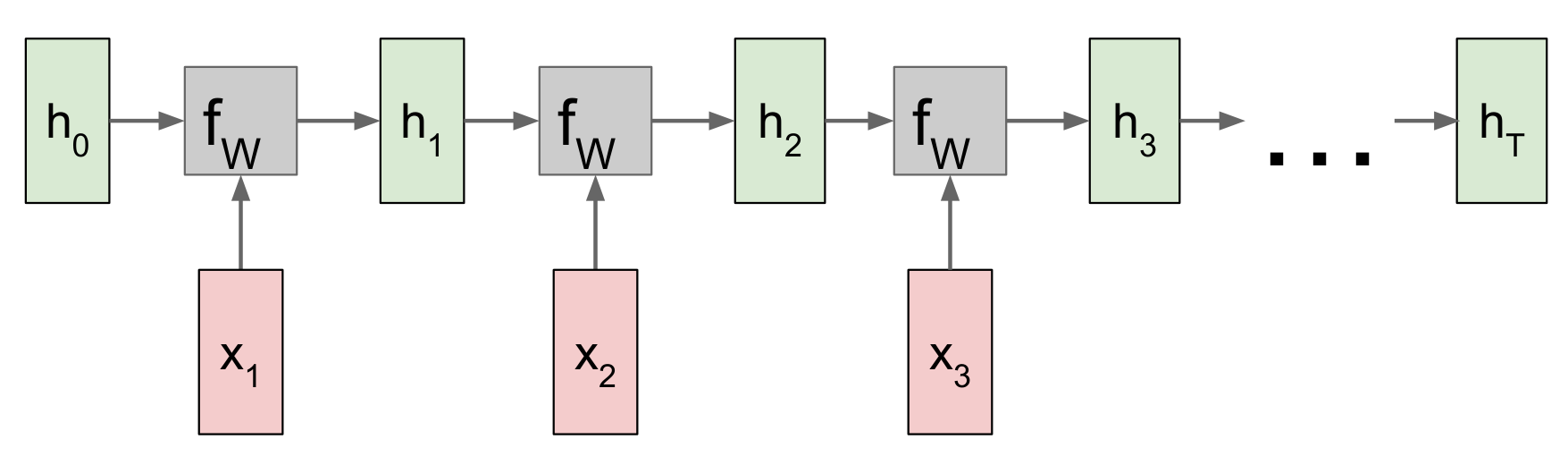
Repeated recurrent functions f_W connect h₀ to h₁, h₂, h₃ and h_T, with one input x at each step.

Read left to right: each cell receives the previous state and the next input. Repeating fW means reusing one learned rule, not learning a new cell at each position.

Source: Stanford University, CS231n · Lecture 10 (4 May 2017), PDF page 25. Fei-Fei Li, Justin Johnson & Serena Yeung. Cropped figure excerpt; original diagram retained. Source details.

05 / WATCH → PREDICT → EXPERIMENT
06 / CHECK YOUR UNDERSTANDING
CHECK 01

If h₁ = 0.8, x₂ = 0 and the scalar recurrence is h₂ = 0.5h₁ + x₂ (no tanh), what is h₂?

Reveal worked reasoning

0.5 × 0.8 + 0 = 0.4. Zero input still allows the previous state to contribute.

CHECK 02

Doubling sequence length while keeping input and hidden widths fixed doubles the number of learned recurrent parameters.

Reveal worked reasoning

False. Parameters are shared across time. The number of cell evaluations grows.

CHECK 03

Which object changes as each new input is read during inference?

Reveal worked reasoning

The hidden state changes. The learned weights stay fixed during an ordinary forward pass.

02
LSTM / SELECTIVE MEMORY

Keep what matters.
Expose what is useful.

01 / THE HOOK

“The keys to the old cabinet beside the window … are missing.” How can “keys” stay relevant through all those intervening words?

KEEP THIS CLUEkeys → plural
IGNORE FOR THIS DECISIONcabinet · window → singular
02 / SEE THE PROBLEM
A distant cueplural subject
Repeated rewritesnew words enter the same summary
A late decisionare, not is
The subject–verb example motivates a dependency. It does not imply that one neuron stores a clean grammatical rule.
03 / EXPLANATION & ANALOGY

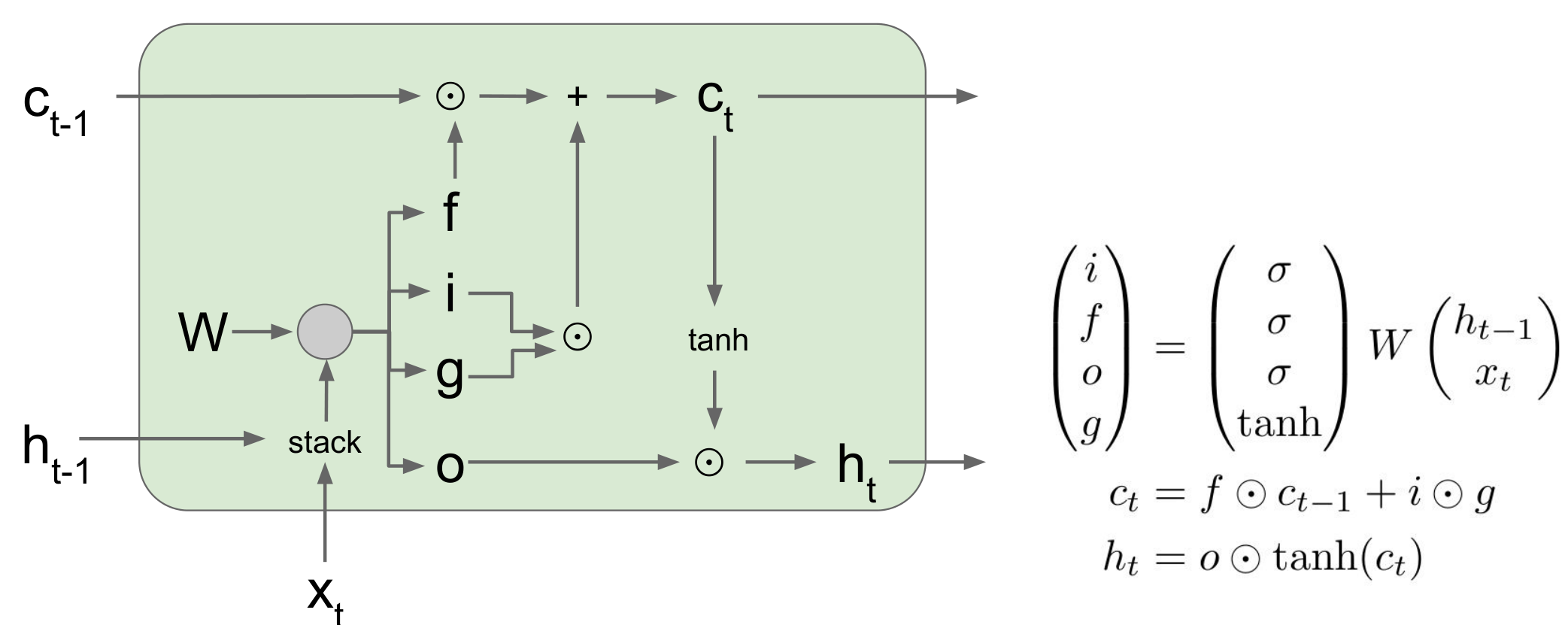
A long short-term memory (LSTM) cell carries two vectors: the cell state cₜ for stored content and the hidden state hₜ for exposed output. A forget gate fₜ scales old memory, an input gate iₜ controls new writing, and an output gate oₜ controls what is exposed. The signed candidate gₜ proposes new content.

Imagine a notebook with three controls: retain part of the old notes, write selected new notes, and open a viewing window onto the page. Closing the window does not erase the notebook. The analogy describes the operations; the model learns continuous, coordinate-wise gates.

A gate is a vector of numbers between 0 and 1, usually produced by a sigmoid. It is not a human rule such as “forget every noun”. Every gate is computed from the current input and previous hidden state using learned weights.

04 / GIVE THE IDEA A RULE
cₜ = fₜ ⊙ cₜ₋₁ + iₜ ⊙ gₜ
hₜ = oₜ ⊙ tanh(cₜ)

⊙ means element-by-element multiplication. All four gate/candidate vectors and both state vectors have H coordinates. f = 1 retains; f = 0 removes the old contribution. i controls writing independently; f + i need not equal 1.

Go deeper · All equations, shapes & a worked coordinate
aₜ = [hₜ₋₁ ; xₜ]
fₜ = σ(Wf aₜ + bf) · iₜ = σ(Wi aₜ + bi)
oₜ = σ(Wo aₜ + bo) · gₜ = tanh(Wg aₜ + bg)

Semicolons inside brackets mean concatenation; dots between equations separate formulas, not multiplication. σ(v) = 1/(1 + exp(−v)). Each W has shape H × (H + d); each bias has H values. Sigmoid produces values strictly between 0 and 1 for finite inputs; sliders include the useful idealized limits.

For cₜ₋₁ = 0.8, f = 0.75, i = 0.5 and g = 0.4, cₜ = 0.6 + 0.2 = 0.8. With o = 0.6, hₜ = 0.6 tanh(0.8) ≈ 0.398. With o = 0, hₜ = 0 while cₜ remains 0.8. The hidden value is neither a class probability nor a stored token.

The cell state is not forced into [−1, 1]; additions can accumulate. The standard hidden state is bounded by its tanh and output gate. This worksheet uses the modern forget-gate form, no peephole connections and no projection. For one bias per affine transform, P = 4H(d + H + 1), excluding a task head.

ARCHITECTURE / UNIVERSITY REFERENCE

Inside one LSTM cell

Open full-size image ↗
An LSTM cell takes previous cell and hidden states plus the input; forget, input and output gates control the cell-state and hidden-state paths.

Follow the upper c path first, then the lower h path. The source’s g is our signed candidate; “stack” means concatenate ht−1 and xt. W combines the four learned affine transforms; biases are omitted in this schematic.

Source: Stanford University, CS231n · Lecture 10 (4 May 2017), PDF page 98. Fei-Fei Li, Justin Johnson & Serena Yeung. Cropped figure excerpt; original diagram retained. Source details.

05 / WATCH → PREDICT → EXPERIMENT
06 / CHECK YOUR UNDERSTANDING
CHECK 04

Using cₜ₋₁ = 0.8, f = 0.75, i = 0.5, g = 0.4, calculate cₜ.

Reveal worked reasoning

Retain 0.75 × 0.8 = 0.6; write 0.5 × 0.4 = 0.2; add them to obtain 0.8.

CHECK 05

If o = 0 while cₜ = 0.8, what is hₜ?

Reveal worked reasoning

hₜ = 0 × tanh(0.8) = 0. The cell state remains 0.8.

CHECK 06

Which idealized settings preserve the old cell exactly for this step, regardless of candidate?

Reveal worked reasoning

f = 1 and i = 0 give cₜ = cₜ₋₁. The output gate separately controls exposure.

03
LSTM / THE LEARNING SIGNAL

A memory route is also
a route for correction.

01 / THE HOOK

An early clue caused a late mistake. If the correction almost disappears on its way back, how will the model learn to preserve that clue?

20 SMALL MULTIPLIERS0.8 × 0.8 × … × 0.8
20 NEAR-ONE MULTIPLIERS0.95 × 0.95 × … × 0.95
02 / SEE THE PROBLEM
Late losshow wrong was the prediction?
Chain rulemultiply local derivatives backward
Early operationhow should its parameters change?
Forward memory and backward sensitivity are related but different quantities. This experiment isolates one route through the computation.
03 / EXPLANATION & ANALOGY

Training uses backpropagation through time: the chain rule sends credit through repeated state updates. Multiplying many small local derivatives can make an early contribution difficult to learn; large factors can instead lead to exploding gradients.

Think of passing a correction through many volume knobs. If every knob turns the message down, the first person barely hears it. The additive LSTM cell route supplies knobs that can be learned near 1, without forcing the old cell content through a new tanh at every link on that route.

Holding gates fixed, the direct edge from cₜ₋₁ to cₜ has multiplier fₜ. A forget gate near 1 can preserve this path. This is a useful mechanism, not proof that the full network has no vanishing gradients.

04 / GIVE THE IDEA A RULE
direct cell-state path: ∏ₖ₌₁ᴸ fₖ
constant f: fᴸ   ·   linear RNN comparison: 0.8ᴸ

For vectors, each direct edge has diagonal Jacobian diag(fₜ). Here L is the number of recurrent links. The displayed product holds gate values fixed and isolates the direct route; total derivatives also include routes through h and the gate computations.

Go deeper · Tanh derivatives, half-life & practical limits

For a scalar vanilla RNN hₜ = tanh(w hₜ₋₁ + xₜ), ∂hₜ/∂hₜ₋₁ = w(1 − hₜ²). Even a weight above 1 may be paired with a small tanh derivative. The interactive comparison removes tanh from its RNN baseline so the two products can be inspected exactly.

With no writes and f = 0.95, an initial cell value retains a fraction 0.95ᴸ. Its half-life is log(0.5)/log(0.95) ≈ 13.5 steps; at f = 0.99 it is about 69 steps. Gate choices and useful timescales depend on the data.

The derivative from cₜ to exposed hₜ also contains oₜ(1 − tanh²(cₜ)). Saturation or a closed output gate can weaken that route even when the cell path preserves information. Gates also depend on prior hidden states. Therefore fᴸ is not the complete gradient of a loss or a parameter.

Gradient clipping limits large accumulated parameter gradients; it does not reconstruct a vanished signal. Truncated backpropagation limits how far training credit travels, even if hidden states are carried farther. LSTM does not remove finite memory, optimization difficulty or sequential computation.

ARCHITECTURE / UNIVERSITY REFERENCE

The cell-state path across several steps

Open full-size image ↗
Three LSTM cells joined by the cell-state path c₀ to c₃, with red arrows pointing backward along that path.

The red arrows trace backward credit along the direct cell-state route. Each crossed forget gate still multiplies that route by f; this is not a guarantee of an unchanged gradient. The interactive below measures this distinction.

Source: Stanford University, CS231n · Lecture 10 (4 May 2017), PDF page 100. Fei-Fei Li, Justin Johnson & Serena Yeung. Cropped figure excerpt; original diagram retained. Source details.

05 / WATCH → PREDICT → EXPERIMENT
06 / CHECK YOUR UNDERSTANDING
CHECK 07

A fixed forget gate is 0.5 for 3 links, with no writing. What fraction remains?

Reveal worked reasoning

0.5³ = 0.125 = 1/8. Repeated retention multiplies, not adds.

CHECK 08

Does a direct-path product near 1 guarantee that every LSTM parameter receives a strong learning signal?

Reveal worked reasoning

No. Other paths, gate dependencies, output saturation and the loss derivative also affect the full gradient.

CHECK 09

Which operation caps an exploding gradient but does not restore a vanished gradient?

Reveal worked reasoning

Gradient clipping rescales or limits large parameter gradients. It does not amplify the missing information in tiny gradients.

04
GRU / A SIMPLER GATED CELL

One notebook.
Two decisions.

01 / THE HOOK

Can we retain old evidence and admit a new proposal without maintaining separate c and h vectors?

LSTMcell memory c + hidden output h
GRUone hidden state h
02 / SEE THE PROBLEM
Old stateuseful carry information
Candidate branchhow much old context should shape a new proposal?
Blendhow much old state should survive?
The reset and update gates answer different questions. Resetting the candidate branch does not necessarily erase the final state.
03 / EXPLANATION & ANALOGY

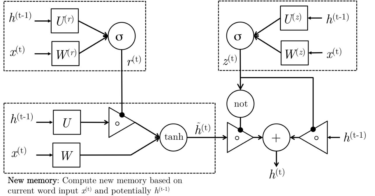
A gated recurrent unit (GRU) combines memory and output into one hidden state. Its reset gate rₜ controls how previous state participates in the candidate. Its update gate zₜ mixes the previous state with that candidate.

Keep one notebook and draft a replacement paragraph on scrap paper. Reset decides how much old context the draft uses. Update decides how much of the old page survives when the draft is merged. Discarding old context from the draft does not force you to discard the old page.

Our convention: z is the fraction of old state retained. Thus z near 1 means “keep”, and z near 0 means “replace with the candidate”. Check the equation in any other reference before interpreting its gate labels.

04 / GIVE THE IDEA A RULE
h̃ₜ = tanh(Wₓxₜ + Wₕ(rₜ ⊙ hₜ₋₁) + b)
hₜ = zₜ ⊙ hₜ₋₁ + (1 − zₜ) ⊙ h̃ₜ

The reset-before-matrix variant is shown. The blend is coordinate-wise: each coordinate has its own r and z. There is no separate output gate or cell-state vector in this GRU.

Go deeper · Learned gates, variants & cost
rₜ = σ(Wr [hₜ₋₁ ; xₜ] + br)
zₜ = σ(Wz [hₜ₋₁ ; xₜ] + bz)

With x = 0.2, old h = 0.8, r = 0.5, weights 1 and bias 0, the candidate is tanh(0.6) ≈ 0.537. At z = 0.75, hₜ = 0.75 × 0.8 + 0.25 × 0.537 ≈ 0.734. At r = 0, the candidate is tanh(0.2), but z = 1 still retains old h = 0.8.

Some references write (1 − z)hₜ₋₁ + z h̃ₜ, so their z means “write”. Some libraries use reset-after-projection, r ⊙ (Wₕh + bₕ), instead of Wₕ(r ⊙ h). These are not generally interchangeable for matrices. Match the implementation before copying weights or counting biases.

With one bias per affine transform, a GRU has P = 3H(d + H + 1), versus 4H(d + H + 1) for this LSTM. At equal H it has 25% fewer recurrent parameters. Frameworks with separate input and recurrent biases change this count. Fewer parameters can reduce storage, but measured speed depends on kernels and hardware; accuracy depends on the task and training.

ARCHITECTURE / UNIVERSITY REFERENCE

Inside a GRU: candidate and carry branches

Open full-size image ↗
GRU reset and update gate networks control a candidate branch and an old-state carry branch; the contributions combine to form the next hidden state.

Trace r into the candidate and z into the carry branch. Here “not” means 1 − z, so z retains old state, as in our worksheet. Variant note: this source places reset after the recurrent projection, r ⊙ (Uh). Our formula uses reset before it, U(r ⊙ h). They coincide in our scalar demonstration, but generally differ for matrices.

Source: Stanford University, CS224n · Lecture Notes V (Winter 2019), Figure 12, PDF page 12. Milad Mohammadi, Rohit Mundra, Richard Socher, Lisa Wang & Amita Kamath. Cropped figure excerpt; original diagram retained. Source details.

05 / WATCH → PREDICT → EXPERIMENT
06 / CHECK YOUR UNDERSTANDING
CHECK 10

Using our convention, z = 1 and old h = 0.8. What is the new h, whatever the candidate?

Reveal worked reasoning

1 × 0.8 + 0 × candidate = 0.8. Our z retains old state.

CHECK 11

If r = 0, what is guaranteed in the GRU variant shown here?

Reveal worked reasoning

The candidate ignores the previous hidden state on its reset branch. The carry term z ⊙ hₜ₋₁ may still retain it.

CHECK 12

For d = 3, H = 2 and one bias per transform, how many GRU recurrent parameters are there? Exclude the head.

Reveal worked reasoning

3H(d + H + 1) = 3 × 2 × (3 + 2 + 1) = 36. The matching LSTM has 48.

05
BIDIRECTIONAL RNNs / CONTEXT & CAUSALITY

The next words
can change the meaning.

01 / THE HOOK

You have only read “the bank”. Would “near the river” and “approved a loan” support the same interpretation?

COMPLETE SENTENCE Athe bank near the river
COMPLETE SENTENCE Bthe bank approved a loan
02 / SEE THE PROBLEM
Forward reader →prefix through the current word
← Backward readersuffix through the current word
Aligned pairtwo contextual views at one position
Changing later words cannot change the forward state already computed at bank. A second pass can incorporate those words when the full input is available.
03 / EXPLANATION & ANALOGY

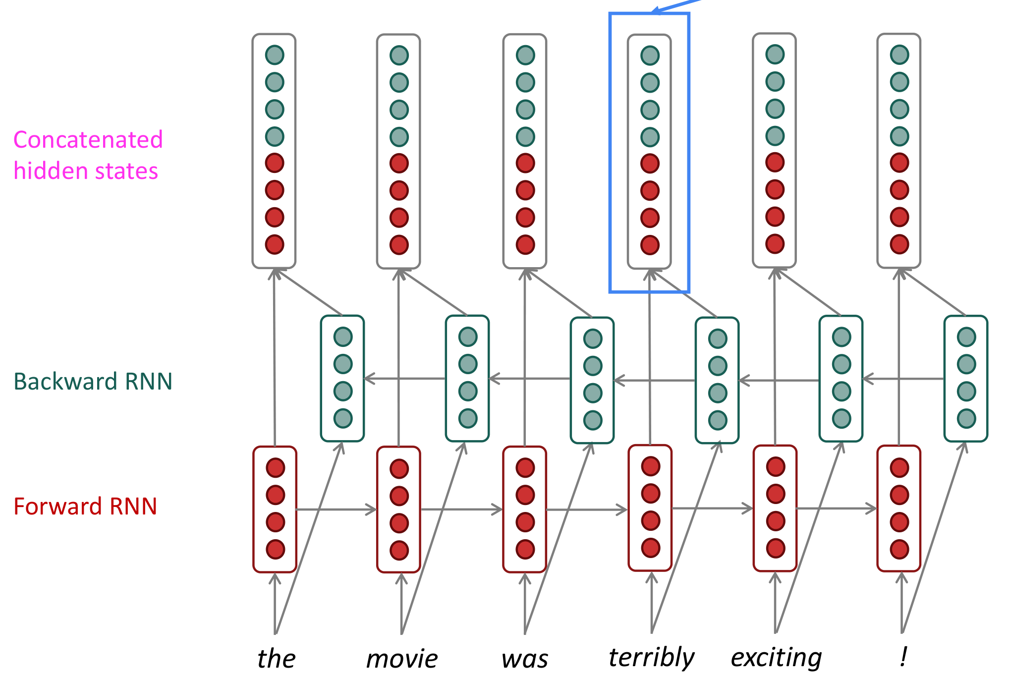
A bidirectional RNN runs two recurrent networks over the same input: one left to right, one right to left. They have separate learned parameters. At a position, concatenate the two states and let a task head use both contexts. Either direction can use a vanilla RNN, LSTM or GRU cell.

Two readers annotate a completed paragraph from opposite ends, then compare notes at the same word. Their meeting point is a token position, not whichever token each happened to process second.

This is useful for tagging a complete sentence, offline speech transcription or encoding a known source sentence for translation. A live predictor cannot use an unseen suffix. A backward pass is a second forward computation over reversed input, not backpropagation.

04 / GIVE THE IDEA A RULE
h→ₜ = F→(xₜ, h→ₜ₋₁)   ·   h←ₜ = F←(xₜ, h←ₜ₊₁)
uₜ = [h→ₜ ; h←ₜ] ∈ ℝ²ᴴ   →   head(uₜ)

The right-to-left state at t depends on positions t through T. The forward state depends on 1 through t. Concatenation keeps both vectors; it does not add them. The boundary states h→₀ and h←T₊₁ are initialized before their respective passes.

Go deeper · Alignment, latency & honest evaluation

For tokens [A, B, C], the backward computation visits C, then B, then A. Store or reorder its results by original token index before pairing forward and backward states. For token B, use [h→₂ ; h←₂], not [h→₂ ; h←₃].

At hidden width H = 4 per direction, each concatenated token representation has 8 features. A full-sequence summary can concatenate h→T with h←₁. Using the backward output aligned to the final token alone does not summarize the whole sequence in that direction. A bidirectional LSTM has 2 × 4H(d + H + 1) recurrent parameters under our bias convention; the head also gets a wider input.

Bidirectionality requires the chosen input window to be available. Offline transcription may use the whole recording; streaming can use a limited look-ahead window at a latency cost. Forecasting may bidirectionally encode a fully observed history window, but must never include the future being forecast. In translation, the whole source can be known while target generation remains causal.

Split related people, recordings or documents by source when appropriate; for forecasting use chronological evaluation and prevent overlapping future targets from leaking. Fit scalers on training data only. Padding is not meaningful time: mask padded outputs in the loss and prevent padded steps from contaminating state (for example, use lengths/packed sequences). Reset states between unrelated sequences. Carry state only when continuity and boundaries are intentional.
ARCHITECTURE / UNIVERSITY REFERENCE

Two readers, aligned at each token

Open full-size image ↗
Separate forward and backward RNN rows process a sentence in opposite directions; states aligned to each word are concatenated above them.

Red features come from the forward reader; teal features come from the backward reader. The top vector stacks both at the same word. These coloured dots represent features, not numerical values; the interactive below supplies a numerical example.

Source: Stanford University, CS224N/Ling284 · Lecture 6 (Spring 2024), PDF page 34. Christopher Manning. Cropped figure excerpt; original diagram retained. Source details.

05 / WATCH → PREDICT → EXPERIMENT
06 / CHECK YOUR UNDERSTANDING
CHECK 13

Each direction has H = 4 features. How wide is the concatenated representation at one token?

Reveal worked reasoning

Concatenation places four forward and four backward values side by side: 2H = 8.

CHECK 14

Which use of a bidirectional model respects the prediction boundary?

Reveal worked reasoning

A completed sentence is already observed. Its later words can inform earlier token labels. The other examples feed unknown targets into their own predictions.

CHECK 15

Which statement describes the backward RNN pass?

Reveal worked reasoning

It computes states from right to left with its own parameters. Backpropagation is the separate training operation that computes derivatives.

06
RETURN TO THE MISSION

What did you keep?
What were you allowed to see?

Recall the opening colour before revealing it at the top. The lesson was never “remember everything”. It was to retain useful information, control new writing and respect the information available at prediction time.

Two independent choices: cell design and reading direction
ChoiceState & controlWhat it changes
Vanilla RNNh; repeated nonlinear updateCompact baseline; long credit paths may be difficult
LSTMc and h; forget, input, output gatesSeparate stored memory and exposed output
GRUh; reset and update gatesFewer affine transforms at equal hidden width
BidirectionalTwo independent recurrent directionsUses both sides of an available input; can wrap any cell above

Design challenge · two products, one team

A. Tag faults in a completed machine recording. B. Raise a fault alert immediately as sensor readings arrive. Both may need clues from far earlier.

Discuss a defensible design

A bidirectional LSTM or GRU is a reasonable candidate for A because the recording is complete. For B, begin with a unidirectional gated model over observed readings; look-ahead would require an explicit delay. Compare LSTM and GRU on held-out machines or recordings with matched data, tuning budget and measured latency. Use chronological evaluation where the use case predicts future operation, fit preprocessing on training data, and prevent related windows from leaking. Neither cell is guaranteed to win.

Keep the next puzzle open. We still compress the past into fixed-size state vectors. What if a prediction could look back at selected earlier states directly? That question leads to attention.

Answers stay in this browser when storage is available. Export a text copy to keep them.

READ FURTHER / ATTRIBUTION

The sources behind the ideas.

The five architecture reference images are cropped excerpts from Stanford University teaching PDFs, credited with authors and exact page links beside each figure. Interactive diagrams, animation storyboards and numerical examples are original teaching assets for this collection. Examples use chosen values; they are not measured training results.

Five reusable SVG figures · Animation storyboards · Teaching notes & pacing